This is an old revision of the document!
Experiment 2: Capacitors
Objectives of the experiment
Getting to know the following components
- Digital multimeter
- Function generator
- Oscilloscope
- Breadboard
electrical-engineering learning outcome in
- generating and displaying periodic signals
- determining capacitances
- measuring the characteristic curve of a diode and a Zener diode
Preparation for the lab
in the ILIAS course
Read the documents for Experiment 2 here.
Display of periodic signals on the oscilloscope
Build the following circuit in figure 1 with the function generator and the oscilloscope.

Fig. 1: Periodic signals on the oscilloscope
Set the signals listed in table 1 on the function generator and draw the corresponding oscilloscope screen images. The signal display on the oscilloscope should optimally fill the screen

Also document the settings of the used channels, the time base, and the GND line on the left side of the screen drawings.
 Fig. 2: Sine, f = 1 kHz, U = 1.8V
Channel 1: $ \frac{V}{\rm DIV} = $
Time basis: $ \frac{T}{\rm DIV} = $
 Fig. 3: Triangle, f = 4 kHz, U = 3 V
Channel 1: $ \frac{V}{\rm DIV} = $
Time basis: $ \frac{T}{\rm DIV} = $
 Fig. 4: Rectangle, unipolar, f = 2 kHz, U = 5 V
Channel 1: $ \frac{V}{\rm DIV} = $
Fig. 4: Rectangle, unipolar, f = 2 kHz, U = 5 V
Channel 1: $ \frac{V}{\rm DIV} = $
Time basis: $ \frac{T}{\rm DIV} = $
 Fig. 5: Rectangle, bipolar, f = 5 kHz, U = 2 V
Channel 1: $ \frac{V}{\rm DIV} = $
Time basis: $ \frac{T}{\rm DIV} = $
 Fig. 6: Sine DC Offset, f = 2.5 kHz, U = 4 V, UDC = 2 V
Channel 1: $ \frac{V}{\rm DIV} = $
Time basis: $ \frac{T}{\rm DIV} = $
Capacitors
Direct capacitance measurement
Capacitors are components that allow the storage of electrical energy. In the charged state an electrical charge is present. This charge causes a voltage at the electrical terminals of the capacitor.
Build the following circuit on the breadboard with three capacitors, s. figure 7:

Measure the capacitance of capacitors $C_{\rm 1}$, $~C_{\rm 2}$, $~C_{\rm 3}$ with the multimeter and enter the measured values in table 2.

Capacitors can be connected in series and/or in parallel. The total capacitance of two or more capacitors in parallel is calculated as:
$$C_{\rm total} = C_{\rm 1} + C_{\rm 2} + ... + C_{\rm n}$$
The total capacitance of capacitors connected in series is calculated as:
$$ \frac{1}{C_{\rm total}} = \frac{1}{C_{\rm 1}} + \frac{1}{C_{\rm 2}} + ... + \frac{1}{C_{\rm n}}$$
Series connection:
- $C_{\rm 1}+ C_{\rm 2}$ (measured between terminals 1 and 3)
- $C_{\rm 2}+ C_{\rm 3}$ (measured between terminals 3 and 4)
Parallel connection:
- $C_{\rm 1~} || ~C_{\rm 3}$ (measured between terminals 1 and 2; wire bridge between 1 and 4)
- $C_{\rm 1~} || ~C_{\rm 2}$ (measured between terminals 1 and 2; wire bridge between 1 and 3)
Series/parallel connection:
- $C_{\rm 1~}+(C_{\rm 2~} || ~C_{\rm 3})$ (measured between terminals 1 and 3; wire bridge between 3 and 4)
Enter the measured and calculated values in table 3.

The built-in capacitors have values from the E6 series. The E6 series for capacities is shown below. For the measured capacities from table 2, determine the matching value from the E6 series and calculate the respective measurement deviation from the nominal value in %.
$$ \text{Deviation} = \frac{C_{\rm meas}-C_{\rm nom, E6 series}}{C_{\rm nom, E6 series}}\cdot 100% $$
Enter your results in the spaces provided below.
$C_{\rm 1~} (E6)~=~ {\rm ....................~} ({\rm Deviation ............}{\%})$
$C_{\rm 2~} (E6)~=~ {\rm ....................~} ({\rm Deviation ............}{\%})$
$C_{\rm 3~} (E6)~=~ {\rm ....................~} ({\rm Deviation ............}{\%})$
The E6 series for capacities in table 4:

RC network
The capacitance of a capacitor is defined as the quotient of charge by voltage: $$ C=\frac{Q}{U} $$
Capacitors must be charged via an electrical source figure 8.

A capacitor charges the faster the smaller the series resistor $R$ is. During charging, the voltage $u_{\rm C}$ results from a differential equation as: $$ u_{\rm C}({\rm t})=U\cdot ({\rm 1}-e^{-\frac{t}{\tau}}), {\rm with~~} \tau = R\cdot C $$
The constant $\tau$ is called the time constant. After this time, the capacitor is charged to approx. ${\rm 63}~{\rm\%}$. The fundamental equation for the relation between current and voltage at a capacitor is:
$$ i_{\rm C}({\rm t})=C\cdot \frac{{\rm d}u_{\rm C}}{{\rm dt}} $$
From the two equations, the current through the capacitor is: $$ i_{\rm C}({\rm t})=\frac{U}{R}\cdot e^{-\frac{t}{\tau}} $$
The graphical representation of voltage and current during the charging of a capacitor over time is shown in figure 9.
 Fig. 9: Voltage/Current in case of charging capacitor
Because of the exponential function, charging is theoretically only complete after an infinitely long time. The capacitor voltage equals ${\rm 63}~{\rm\%~} U$ after ${\rm 1}\cdot \tau$, ${\rm 86}~{\rm\%~} U$ after ${\rm 2}\cdot \tau$, ${\rm 95}~{\rm\%~} U$ after ${\rm 3}\cdot \tau$, ${\rm 98}~{\rm\%~} U$ after ${\rm 4}\cdot \tau$, and ${\rm 99}~{\rm\%~} U$ after ${\rm 5}\cdot \tau$. It is assumed that the capacitor is fully charged after a time span $T = {\rm 5}\cdot \tau$ and the voltage across the capacitor has reached $U$. If the charged capacitor $C$ is discharged through a resistor $R$, the solution of the differential equation for the voltage is:
$$ u_{\rm C}({\rm t})=U\cdot e^{-\frac{t}{\tau}} $$
For the current accordingly:
$$ i_{\rm C}({\rm t})=- \frac{U}{R}\cdot e^{-\frac{t}{\tau}} $$
Now build the following circuit. Connect the function generator and the oscilloscope to the circuit as shown in figure 10.
 Fig. 10: Circuit with oscilloscope + function generator
Connect the function generator’s ground (black) to point 2 and the signal lead to point 1. For the oscilloscope connection use the BNC‑banana adapter; the red socket is the signal input and the black socket is the ground connection to the oscilloscope. Connect Channel 1 to point 3, Channel 2 to point 4, and ground to point 5. You only need to make the ground connection to the oscilloscope once, since the ground lines are connected inside the oscilloscope.
Enter in table 5 both the measured values of the components used and the calculated time constant $\tau$.

Set the voltage $u_{\rm F}$ generated by the function generator to a unipolar square with amplitude 5 $V$ (i.e., no negative signal voltages occur!). The frequency on the function generator must be chosen so that the capacitor just fully charges and then fully discharges again.
Calculate the frequency to be set:
$f_{\rm 1} =~{\rm ...............}$
Sketch the voltages measured with the oscilloscope for $u_{\rm F}$, $u_{\rm C}$, and $u_{\rm R}$ in the following screen diagram. Also enter alongside the screen drawings the set $\frac{V}{\rm DIV}$ of the channels and the $\frac{T}{\rm DIV}$ of the time base.
Channel 1: $ \frac{V}{\rm DIV} = $
Channel 2: $ \frac{V}{\rm DIV} = $
Time basis: $ \frac{T}{\rm DIV} = $
Draw tangents in the screen diagram for the start of charging and the start of discharging.
What is the charging current or discharging current at the beginning?
${\rm ........................................................................................}$
${\rm ........................................................................................}$
The circuit is now to be operated at higher frequencies. Set the frequency to:
- $f_{\rm 2} = ~{\rm 10}\cdot f_{\rm 1}$
- $f_{\rm 3} = ~{\rm 100}\cdot f_{\rm 1}$
Measure the waveforms for $u_{\rm F}$, $u_{\rm C}$ and document the results in the following table 6:

Explain your observations for the measurements with $f_{\rm 2}$, $f_{\rm 3}$:
${\rm ........................................................................................}$
${\rm ........................................................................................}$
${\rm ........................................................................................}$
${\rm ........................................................................................}$
Function generator
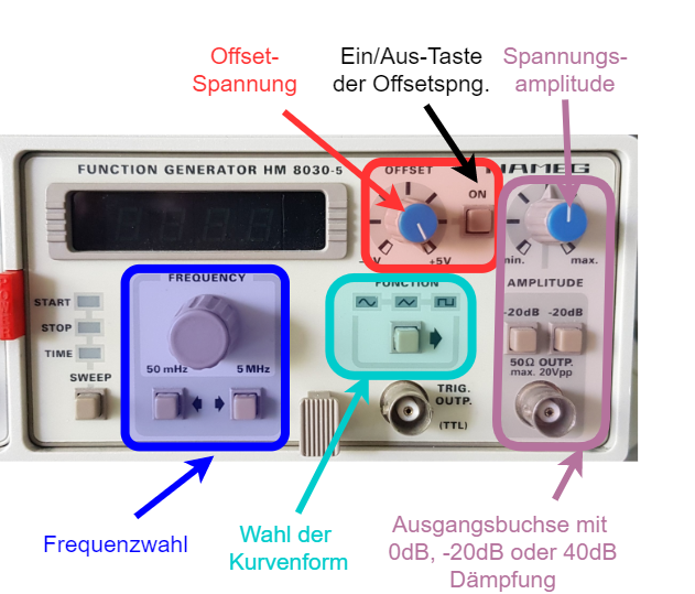
A function generator provides a variable voltage source. In general, these signals can be generated with different waveform shapes, frequencies, and amplitudes. These values can be adjusted on real function generators. In contrast to an ideal function generator, the output current of a real system is limited. As with a real voltage source, an output impedance is specified here.
In figure 17 the function generator used in the lab is shown. It has an output impedance of $50~\rm \Omega$. In the following, the settings are briefly described:
- The waveform can be selected using the FUNCTION button. Pressing the button selects the next waveform. At start-up, the sine waveform (∿) is selected; the following waveforms are: triangle and square or pulse. The waveforms can be seen in the simulation below; a sawtooth signal is not possible with this function generator.
- The frequency can be changed via two inputs
- The potentiometer under FREQUENCY allows precise adjustment. Turning clockwise increases the frequency.
- Using the buttons under the potentiometer, the frequency can be changed by one decade—i.e., by a power of ten—down (button with arrow to the left) or up (button with arrow to the right). The limits are $50~\rm mHz$ and $5~\rm MHz$.
- There are also several controls for the voltage
- The potentiometer OFFSET allows precise selection of the DC component. To enable a DC component, press the ON button.
- At the output jack, two attenuations of $-20~\rm dB$ can be switched on. This reduces the peak-to-peak voltage range from [$0~\rm V$, $10~\rm V$] to [$0~\rm V$ , $1~\rm V$ ] or [$0~\rm V$ , $0,1~\rm V$ ].
- The AMPLITUDE, i.e. the peak-to-peak voltage, can be finely adjusted using a potentiometer.
Oscilloscope used
Even before the digital multimeter, the oscilloscope is the most important measuring instrument in electrical engineering and electronics. It makes it possible to display a voltage waveform u(t) over time t, observe it in “real time,” and measure it. In many experiments and analyses, it is a central component because it can make electrical processes visible. In addition to quantitative statements (how high is the voltage and when?), it is also helpful for qualitative results (for example: Is there a fault in the circuit?).
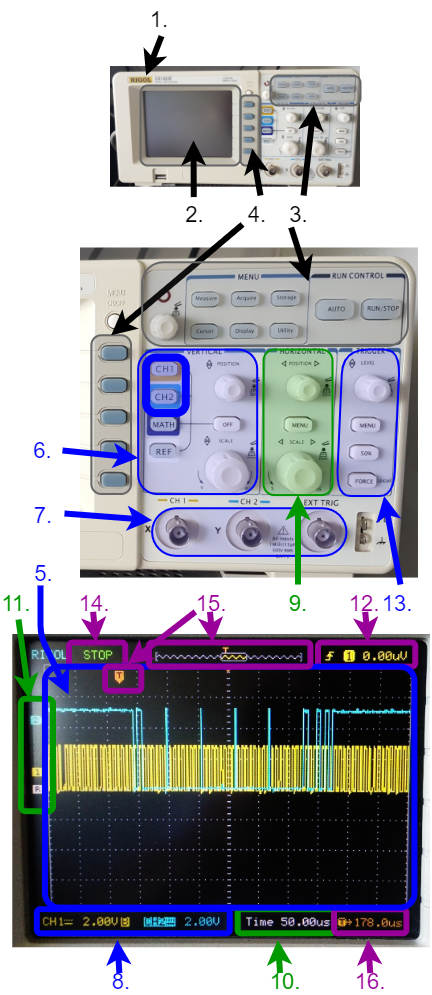
Good knowledge of the oscilloscope is necessary for this experiment. In figure 18 you can see the control panel of the DS1052E used, which is briefly described here.
Please use the buttons marked with “ ” to learn more about the individual functions
- On/off switch (1.)
- Display area (2.)
- Selection of operating modes (3.)
- Menu selection buttons (4.)
- The oscilloscope can be turned on/off using the button on the top (1.)
- In the display area (2.) information is shown in the user interface after switching on, which is explained below
- At the top right (3.) two operating modes can be selected: single acquisition after a trigger signal (
RUN/STOP) and automatic selection of various settings (AUTO). In addition, there are various menu selection buttons there, e.g. for the cursor menu (3.). - In the menus, displayed functions can be selected via five selection buttons (4.). The menus are not discussed further below.
- Display window (5.)
- Channel selection / horizontal controls (6.)
- Input jacks (7.)
- Channel coupling / voltage scale (8.)
- The largest area is the display window (5.). The display window shows 10 horizontal and 8 vertical divisions (eng. divisions, abbreviation Div.). As a rule, the voltage-time waveform is shown here.
- In the figure, two waveforms are displayed simultaneously: channel 1 in yellow and channel 2 in mint. These can be switched on/off using the channel selection (6. top two buttons).
- The signals are fed in via the input jacks (7.) (CH 1 : channel 1, CH 2 : channel 2)
- For the signal, you can choose whether the DC component is suppressed (AC coupling) or not (DC coupling). The channel coupling is shown in the display (8.) as a line (
=for DC coupling) or a tilde (~for AC coupling)
- vertical controls (9.)
- horizontal controls (6.)
- voltage scale (8.)
- time base (10.)
- signal mean values (11.)
- The voltage scale can be varied using the vertical controls (9.): POSITION shifts a waveform up/down. SCALE enlarges/reduces the vertical axis (= voltage axis).
- The same can be done for the time axis using the horizontal controls (6.): it can also be shifted with POSITION and enlarged/reduced with SCALE.
- The current scaling can be read from the display area: In the image, a voltage scale of
2.00 V/Divfor both signal waveforms (8.) and a time base of50.00 us/Div(10.) are shown. - The signal mean values are drawn to the left of the waveform (11.) as a small yellow arrow (channel 1) and a mint-colored arrow (channel 2). If a signal is above or below the displayed area due to incorrect scaling, the corresponding arrow is also shown at the top or bottom edge.
- Display of the trigger threshold at signal mean values (11.)
- Trigger threshold, trigger source (12.)
- Trigger level (13.)
- Acquisition status (14.)
- Position in memory (15.)
- Trigger delay (16.)
- As a rule, acquisition should be triggered when a certain threshold is exceeded or fallen below. This threshold is called the trigger threshold.
- The trigger threshold, trigger source (CH1 or CH2), and triggering on an exceedance (rising edge
͟ ↑͞) or falling below (falling edge͞ ↓͟) can be seen in the display area (12.). The threshold is additionally marked to the left of the waveform (11.). - The knob (13.) can be used to shift the threshold (trigger level). Pressing
50%sets the trigger to the center. - The acquisition status (14.) is located at the top left of the display area.
STOPmeans a still image is shown. When running,T'Dfor triggered is shown here. - The oscilloscope records a longer time period than the one displayed. The displayed position in memory (15.) is shown at the top of the display area. The trigger point is also drawn there. How many (nano-, micro-, or milli-)seconds the trigger point is currently shifted from the displayed center is shown at the bottom right (16.).
On the left you will find a nice introductory video. Note that the specific operation often depends on the manufacturer and model. However, the concepts are the same for all devices.
Virtual oscilloscopes
A virtual oscilloscope can be found on the pages of Aachen University. Try there to “oscilloscope” various function generator settings, e.g.:
- $200~\rm Hz$, sine, offset $1~\rm V$, amplitude $5~\rm V$
- $200~\rm Hz$, square, offset -$1~\rm V$, amplitude $3~\rm V$
What happens if the trigger level is set too high?
Preparation for the oral short test
For this experiment you should
- be able to apply and explain the following concepts:
- periodic signal
- characteristic quantities in the signal-time waveform
- peak value (amplitude)
- peak-to-peak value
- arithmetic mean value
- RMS value (quadratic mean)
- rectified mean value
- period duration
- frequency
- creating the time waveform of a periodic signal
- graphical determination of the above quantities from the time waveform of a signal
- capacitance $C$
- behavior of current $i$ and voltage $u$ across $R$ and $C$ with a rectangular input voltage for $t=[0; \infty]$
- $i_{C,stat}$ and $u_{C,\rm stat}$ in steady state
- time constant $\tau$
- determination of $R$, $C$, $\tau$, $i_{C,\rm stat}$ and $u_{C,\rm stat}$ from the time waveform